STIPS Basic Tutorial
This page will take you through the process of creating a basic STIPS observation. You must have STIPS installed –– if you do not, please see installing STIPS.
Importing STIPS and Checking the STIPS Environment
In order to use STIPS, you must have several sets of data files installed (installing STIPS contains instructions on how to do this). In order to test your STIPS installation, STIPS includes an environment report utility that shows which version of STIPS you have installed, as well as the versions of the most important support packages that STIPS uses. When you run the code below, you should get an output set of the following form:
import stips
print(stips.__env__report__)
STIPS Version x.y.z with Data Version x.y.z at /Some/Path/To/stips_data

STIPS Grid Generated with x.y.z

Pandeia version a.b.c with Data Version a.b.c. at /Some/Path/To/pandeia_refdata

STPSF Version d.e.f with Data Version d.e.f at /Some/Path/To/stpsf_data_path
Setting Up Some Basics
STIPS allows you to set up some basic elements of your observation and pass them when creating and running observations. Below is one way to set these up.
obs_prefix = 'notebook_example'
obs_ra = 150.0
obs_dec = -2.5
Creating a Scene to Observe
STIPS contains functions to generate stellar populations as well as background galaxies.
These functions are all present in the SceneModule class. In order to know what sort
of populations to generate, the Scene Module requires input dictionaries to specify
population parameters. In this example, we will create the following:
A stellar population representing a global cluster with:
100 stars
An age of 7.5 billion years
A metallicity of -2.0
A Salpeter IMF with alpha = -2.35
A binary fraction of 10%
A clustered distribution (higher-mass stars closer to the population center)
An inverse power-law distribution
A radius of 100 parsecs
A distance of 10 kpc
No offset from the center of the scene being created
A collection of background galaxies with:
10 galaxies
Redshifts between 0.0 and 0.2
Radii between 0.01 and 2.0 arcsec
V-band surface brightness magnitudes between 28 and 24
Uniform spatial distribution (unclustered) over 200 arcsec
No offset from the center of the scene being created
Note
Background galaxies are available in STIPS, but are neither supported nor tested.
obs_prefix = 'notebook_example'
obs_ra = 150.0
obs_dec = -2.5

from stips.scene_module import SceneModule

scm = SceneModule(out_prefix=obs_prefix, ra=obs_ra, dec=obs_dec)

stellar_parameters = {
                      'n_stars': 100,
                      'age_low': 7.5e12,
                      'age_high': 7.5e12,
                      'z_low': -2.0,
                      'z_high': -2.0,
                      'imf': 'salpeter',
                      'alpha': -2.35,
                      'binary_fraction': 0.1,
                      'clustered': True,
                      'distribution': 'invpow',
                      'radius': 100.0,
                      'radius_units': 'pc',
                      'distance_low': 20.0,
                      'distance_high': 20.0,
                      'offset_ra': 0.0,
                      'offset_dec': 0.0
                     }

stellar_cat_file = scm.CreatePopulation(stellar_parameters)
print("Stellar population saved to file {}".format(stellar_cat_file))

galaxy_parameters = {
                     'n_gals': 10,
                     'z_low': 0.0,
                     'z_high': 0.2,
                     'rad_low': 0.01,
                     'rad_high': 2.0,
                     'sb_v_low': 30.0,
                     'sb_v_high': 25.0,
                     'distribution': 'uniform',
                     'clustered': False,
                     'radius': 200.0,
                     'radius_units': 'arcsec',
                     'offset_ra': 0.0,
                     'offset_dec': 0.0,
                    }

galaxy_cat_file = scm.CreateGalaxies(galaxy_parameters)
print("Galaxy population saved to file {}".format(galaxy_cat_file))
Creating a STIPS Observation
Once a scene has been created, it’s possible to observe that scene as many times as you wish (and from as many places as you wish, although obviously any observation that doesn’t include at least some of the scene will simply be an empty exposure). In this case, we will create a single Roman WFI observation.
STIPS uses a bit of specialized terminology to describe its observations. In particular:
An observation is a set of exposures with a single instrument (e.g. Roman WFI), one or more filters (where each exposure in the observation will be repeated for every included filter), and some number of the instrument’s detectors (for WFI, between 1 and 18), where each exposure will be repeated, with the appropriate inter-detector offset, for every included director, a single chosen sky background value, a single exposure time (applied to each exposure in the observation), and one or more offsets.
An offset is a single telescope pointing. For each offset specified in the observation, an exposure will be created for each detector and each filter at the offset. STIPS may, optionally, create one or more mosaics at each offset, with a single mosaic including all detectors with the same filter. In addition, STIPS can create a single combined mosaic for each filter in the combined Observation.
In this case, we will create an observation with:
Roman WFI F129
1 detector
No distortion
Sky background of 0.15 counts/s/pixel
The ID 1
An exposure of 1000 seconds
We will use a single offset with:
An ID of 1
No centering (if an offset is centered, then, for a multi-detector observation, each detector is centered on the offset co-coordinates individually rather than the instrument as a whole being centered there)
No change in RA, DEC, or PA from the center of the observation
We will use the following residual settings:
Flatfield residual: off
Dark current residual: off
Cosmic ray removal residual: off
Poisson noise residual: on
Readnoise residual: on
from stips.observation_module import ObservationModule

offset = {
          'offset_id': 1,
          'offset_centre': False,
          'offset_ra': 0.0,
          'offset_dec': 0.0,
          'offset_pa': 0.0
          }

residuals = {
             'residual_flat': False,
             'residual_dark': False,
             'residual_cosmic': False,
             'residual_poisson': True,
             'residual_readnoise': True
            }

observation_parameters = {
                          'instrument': 'WFI',
                          'filters': ['F129'],
                          'detectors': 1,
                          'distortion': False,
                          'background': 0.15,
                          'observations_id': 1,
                          'exptime': 1000,
                          'offsets': [offset]
                          }

obm = ObservationModule(observation_parameters, out_prefix=obs_prefix, ra=obs_ra, dec=obs_dec, residual=residuals)
Finally, nextObservation() is called to move between different combinations of offset and
filter. It must be called once in order to initialize the observation module to the first
observation before adding catalogues.
obm.nextObservation()
Observing the Created Scene
In order to observe the scene, we must add the scene catalogues created above to it, add in error residuals, and finalize the observation. In so doing, we create output catalogues which are taken from the input catalogues, but only contain the sources visible to the detectors, and convert source brightness into units of counts/s for the detectors.
output_stellar_catalogues = obm.addCatalogue(stellar_cat_file)
output_galaxy_catalogues = obm.addCatalogue(galaxy_cat_file)

print("Output Catalogues are {} and {}".format(output_stellar_catalogues, output_galaxy_catalogues))

obm.addError()

fits_file, mosaic_file, params = obm.finalize(mosaic=False)

print("Output FITS file is {}".format(fits_file))
print("Output Mosaic file is {}".format(mosaic_file))
print("Observation Parameters are {}".format(params))
Showing the Result
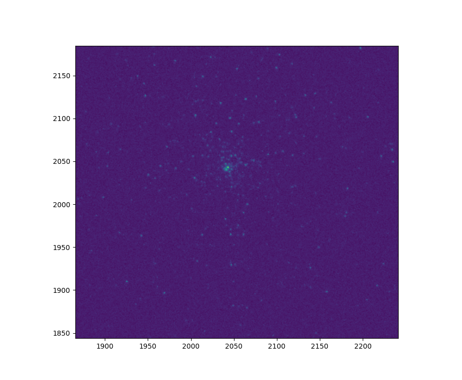
Fig. 1: Output from running the STIPS basic tutorial code. Detail from detector center.
We use matplotlib to plot the resulting simulated image.
import matplotlib
import matplotlib.pyplot as plt
from astropy.io import fits
matplotlib.rcParams['axes.grid'] = False
matplotlib.rcParams['image.origin'] = 'lower'

with fits.open(fits_file) as result_file:
  result_data = result_file[1].data

fig1 = plt.figure()
im = plt.matshow(result_data)
Alternatively, you can open the final .fits file in your preferred imaging software.